
Classes
Many analyses allow you to assign color, size, or other display properties to illustrate your data by generating value classes. This involves summarizing data in groups (so-called classes), and assigning the same display styles to each group.
Numeric and Alphanumeric Classification
The data type determines the evaluation of the value classes. The data type determines the evaluation of the value classes. You can see the data type in the selection list of the Column ("A" stands for alphanumeric columns,"1" for numerical columns). If you have selected a numeric column, the classifcation is based on numeric principles. However, if you have selected a column with the data type "Text", the evaluation is carried out lexically (according to dictionary sorting).
Note: For example, if a column that actually contains numbers is accidentally not marked as a number column during data import, EasyMap treats it like "text" and also sorts numbers lexically! A value class from 4 to 10 would then, for example, include the value 16!
Methods for Creating Classes
There are numerous methods for calculating value classes in statistics. In EasyMap you can use the most common methods:
Here the value classes can be freely defined by the user.
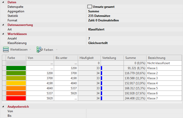
EasyMap calculates the limits of value classes in such a way that approximately the same amount of data records fall into each class.
This form of classification is not only available for numerical columns, but also for columns containing text. EasyMap generates a value class for every occuring text value. This only leads to meaningful results where the number of varying data values is limited. The method is frequently applied for conducting A-B-C customer analyses.
Let EasyMap determine the limit values of the value classes so that all classes have the same width (that is, the difference between the upper and lower class limits is the same for all classes).
EasyMap selects the average value as the boundary between value classes. This is, of course, only possible when only two value classes are generated. The interpretation of this classification is clear: the lower value class contains below-average data, the upper class contains above-average data.
Note: In earlier EasyMap versions (up to 10.0), this classification type was called the "mean value".
The option Sum equal leads to classes whose value class sum is approximately equal. This means that all values falling into one class sum up to a similar sum as the summed values of the other classes. The potential or data volume contained in the individual classes is therefore the same. As a result, value classes with higher values contain only a few data records, while value classes with lower values contain many data records (to arrive at the same sum).
This Classification option is perfect for determining "Priority" areas. You can highlight, for example (preferably few) areas where 25% of sales has already been achieved. On the other hand, such areas can be neglected, because 75% of sales can be achieved with only few areas while the remaining 25%, would have to be added to a very large area.
Example: Pareto distribution (80-to-20 rule)
The "80-to-20-rule" states that most often 20% of market coverage is suffi-cient to cover 80% of the total volume/ Revenue, e.g.: with just 20% of cus-tomers, 80% of sales can be achieved, or by operating 20% of market areas, 80% of customers’ needs are met.
You can solve such problems by a clever classification. Select 5 number of classes. Use the Same Sum classification. Select for the first class value a not deep color, for example, white. Use for the other value classes significantly different colors.Already in the classification dialog box, you can see the rule (Pareto Distribution) applied on the available data. The first couple of class values should contain at least 80% of all cases (Frequency column). If you display the analysis now, the areas that you need to at least get 80% of sales are shown in the map. The white areas show the remaining 20% of its sales.
For the classification type normal distribution (Gauss), the class boundaries are aligned using the parameters of the Gauss normal distribution (mean value μ and standard deviation σ). The class width is set to the standard deviation. If the number of classes is even (recommended), the limit between the two mean value classes is set to the mean value. If the number of classes is odd, the mean value class is centered on the mean value. For two classes, the option normal distribution (Gauss) results in the same value classes as the option mean.
In the case of an even number of value classes generated with the Normal (or Gaussian) distribution option, the following applies for normally distributed values (provided the value classes are completed):
- Approximately 68% of all values fall into the two middle classes
- Approximately 95% of all values fall into the four middle classes
- Over 99% of all values fall into the six middle classes
With the classification type normally distributed (Gaussian) EasyMap always sets the lowest value class open at the bottom and the highest value class open at the top. This ensures that all values are always classified; the outermost value classes contain the extreme values or outliers.
Tip: If you wish to create only closed value classes, raise the number of classes by two before applying Normal (or Gaussian) distribution and subsequently delete the lowest and highest classes.
Note: With automatically generated value classes, it can happen that value classes are omitted due to the data situation. If you have put a lot of effort into the properties of the value classes (for example, defining the design characteristics, descriptions), we recommend that you set the classification type to user-defined so that nothing can change in the value class structure. However, dynamic adaptation to data changes will then no longer take place.
The value class list
The value class list displays each value class as a row. There is always a remainder class that determines the display of unclassified values (these are all values that do not fall into any of the defined classes). Furthermore, there is always at least one correct value class.
If an automatic value class calculation is active (that is, a classification type other than user defined) and you make manual changes to the value classes, the classification type automatically jumps to user defined.
Class List Columns
| Display features | The columns displayed in the value class list are variable. With differentiated analyses, only one design characteristic (e.g. color) is always displayed in the first column; with simple analyses, all design characteristics concerned (2-3) are displayed in the first 2-3 columns. The design characteristics can be edited by double-clicking in the respective cell. |
| Value class limitations |
Normally there is a From and a Up to column where you can set the interval that covers the value class. While the first value still falls into the value class, the last value does not. However, if you use the classification type Attribute, only one column Value is displayed. A data value falls into this class if it is equal to this value. You can also define open classes. In this case, the interval is limited to only one side. To do this, enter * in the cell or delete the value. You can also open both boundaries, so that all values fall into this class. |
| Frequency | This shows how many data records falls into each of the value classes for the current setting. |
| Sum | This displays the sum of all the data records that fall into each of the value classes for the current setting. The column is only displayed for summarizable data and not when using the classification type Attribute. |
| Caption | You can specify an alternative name for the value class that can be used in legends. |
Note: You can also enter multi-line texts. You can use one of the following shortcuts to insert a line break: Shift+Return, Ctrl+Return or Alt+Return.
Sorting the Classes
The columns of the class list can be sorted to change the order in legends. The value classes are then also processed in a different sequence.
A data value is always assigned to the first matching value class!
Analysis area
Usually EasyMap takes into account all data values (i. e. the value range from minimum to maximum) when creating equally distributed and equidistant classes. However, if, for example, you do not want extreme values to be taken into account when calculating value classes, you can do this by specifying an analysis area.
Editing Classes
The various layout attributes of value classes, the boundaries of the individual value classes or the caption of the classes for the legend can be adjusted individually. To do this, simply click in the field that you want to change and select a different symbol or enter a different value for the class boundary.
Note: To change several objects at the same time, press the Ctrl key and select the corresponding fields in the list.
For editing and saving classes, colors, size/width etc., EasyMap also offers various functions that simplify the editing of classes.
| Load value classes | Load the saved settings from another workbook. |
| Save value classes | You can save your settings for a value class (class range limits, colors, class labels, etc.). |
| Smooth Class Range Limits | The set class limit values can be rounded up or down here. Please note that the set classification will then be changed to user-defined and the frequencies recalculated. |
| Allow Gaps | Use this function to set the class limits in such a way that the last value in a class is not the first value of the next class. In doing so, individual values can be removed from the display. |
| Share value classes | The command divide value class divides the marked value class into two, can also be used to easily create symmetrical value classes around the mean value. First select the classification mean, then split the two value classes and get four value classes, where the limit between the second and third class is the mean value. |
| Combine value classes | Using the Merge Classes command allows you to create a new class, by automatically merging several existing classes. At least two classes must be selected before executing this command. As a result, the classification mode automatically switches to User-Defined, and frequencies are immediately recalculated. |
| Remove value classes | You can use this function to delete individual classes. Please note that you must first select the class to be deleted and only then select the command. You can also delete the value class directly from the keyboard (key Delete). The values of the deleted class are added to the Not classified class. |
| Copy Classification | Copy the classification directly to the clipboard. |
| Insert Classification | Insert the classification directly from the clipboard. |
| Select symbol set... |
If you have many value classes that are to be represented by different icons, you can use predefined symbol sets. This saves the manual selection of symbols for each value class. To select a particular symbol set, click on the "symbols" above the value class. Some symbol sets are optimized for a certain number of classes. If there is a greater or lesser number of classes, the system displays a message asking whether the number of classes should be adjusted or not. |
| Save symbol set... | You can also save symbols that you have assembled yourself. |
| Reverse order | Use this command to reverse the sequence of symbols. |
| Load Colors... |
Load saved colors. EasyMap not only offers the possibility to save and reload your own color palettes, but also a wide range of predefined color palettes to choose from. To use one of the color palettes for area shading or for a Boston Grid analysis, click the menu Colors > Load Colors and select a Color Palette from the directory. You may choose from divergent, qualitative and sequential color palettes. Special color palettes for Boston Grid analyses are located in the Boston Grid Matrix subdirectory. You can get a quick overview of the color combination in the Windows Explorer - just set the view in the respective directory to thumbnail view. |
| Save Colors... | Save the set colors as a file for further use. |
| Edit Color Gradient... | Here you can set the set color gradient by specifying two or three colors. Please note that the setting with three colors is only possible from three value classes. |
| Generate Random Colors... | Here you may generate a mixed color palette setting a certain brightness and saturation. |
| Reverse Color Gradient | This command reverses the selected gradient. |
| Create Asymmetrical Color Gradient... |
This is particularly useful in cases where class range limits are asymmetrical (e.g. -100 to -10 / -10 to 10 / 10 to 200 / 200 to 500 / 500 and more). Note: If you want an asymmetric gradient, proceed as follows: Select Edit gradient and then Gradient with specification of 3 colors . Then select the value class to which you want to assign the middle gradient color, and then choose Generate Asymmetric Gradient . |
| Set color effect and transparency... | Here you can adjust the transparency of the colors using a slider or by entering a value. |
| Edit Size Gradient... | You can use this function to determine the size for the smallest and largest value class. |
| Reverse Size Gradient | This function allows you to reverse the size progression with a single click. |
In certain situations, EasyMap displays warnings in the value class list to alert you to potentially unintended situations:
- The value for "From" must be smaller than the value for "Up to": No value would fall into this class. You should correct the class boundaries.
- There is more than one value class whose lower/upper limit is open: In this case, the first value class found would always "win" for very small or very large values.
- The value range of this class overlaps the value range of another class: This can only happen if "Allow Gaps" is activated. The warning indicates that the value class intervals of two classes overlap. In this case, the first value class identified would always "win".
Save and load value classes
In the menu value classes you can save your settings of the value classes (class boundaries, colors, class names etc.) and load them again for further analyses. This is useful, for example, if you need to create a series of similar, comparable maps with different selections. Such a value class file (*.xml) can be reloaded with Load value classes....
