
Area Hatching
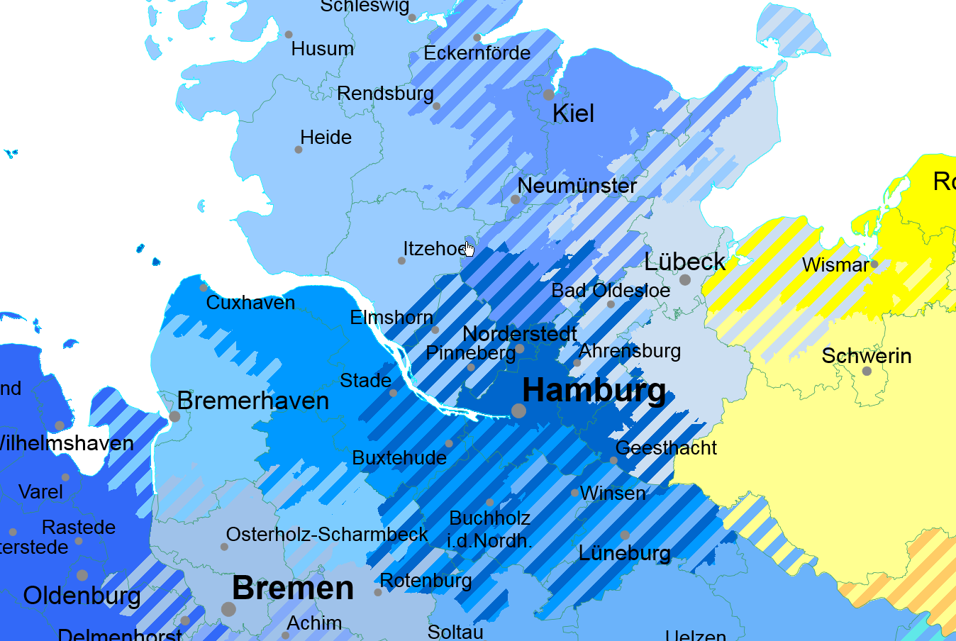
While the standard area shading can only represent one data value per area, the Area hatching analysis offers the possibility to display several data entries per area simultaneously.
Prerequisite for such an analysis and presentation of the data is the existence of several different data sets for the same areas. An example of this type of analysis is the visualization of the election results or the overlapping of employee sales territories.
Note: In this analysis, make sure that the number and width of hatchings are not too large, as otherwise the clarity of the presentation may suffer.
Creating the analysis and selecting the data basis
You insert the analysis via the menu Analyses > Area hatching. You will first be asked to determine the data basis for the analysis and to link it to the map.
Further information is available here.
- What does the Assignment result tell you?
- You can use the Advanced button to specify whether the analysis should take an existing clip map display into account when calculating classifications - more about the analysis reference.
Determining the properties of area hatching
When inserting a new area hatching, all areas for which a data set exists in the selected table are first colored uniformly in the map. The Color and Hatch Width of the area hatching can now be edited in the opening Properties window. You can also access the properties if you want to edit existing analyses.
The colours of area hatching
The color of the hatches is always controlled by a data column:
- First select the data column be evaluated in colors tab of the properties of the analysis. The colors of the area hatching can be either classified, continuous (only with Number columns) or differentiated by a given color value (adjustable during data evaluation).
The width of the area hatching
The width of the area hatching can either be set independently of the data or controlled by means of a data column.
If the hatch width is not data controlled, a maximum of one bar per contained value class is drawn per area. If several values belonging to one area fall into the same color value class, only one color bar is drawn for these values (qualitative display).
Example: Three values belong to an area, two of which fall into a red value class and one value into a yellow value class, the area is hatched red-yellow, whereby the red and yellow bars have the same width.
- Under hatch width, enter the desired width in pixels.
However, if the hatch width is data-controlled (this also applies if only one value class is available), one bar is generated per value (quantitative display). In this case, bars of the same color (bars whose values fall into the same color value class) are placed next to each other. The width of the resulting total bar is the sum of the widths of the individual bars.
Example: If two values of an area each lead to a red bar, and the first bar is 1 cm wide and the second bar 0.5 cm wide, a 1.5 cm wide red bar is displayed. All other colored bars are displayed next to it.
- First, always select the Column in the section Hatching Color and the Hatch Width .
- The hatch width can be differentiated depending on a data value classifiedor proportional. Please enter the width via the number of pixels per strip.
- Classified: By creating value classes, you can define the width of the hatching for a value interval.
- Proportional: You can specify a continuous width curve, which is calculated directly from the analyzed data value using a factor.
- As with the property characteristics you can limit the analysis area or define a color gradient outside of the analysis area.
Determine the details of the analysis
In Details you define other (non-data-dependent) properties of the analysis.For example, set the alignment of the hatching (horizontal, vertical, oblique, etc.).
| Visibility | |
| General |
Here you can control the visibility of objects and elements. |
| Scale range |
Here you can set whether the selected object or plane should be visible at each scale. Or you can specify the scale or zoom level at which the object or layer is visible. |
| In reports |
In Reports there is the possibility to change the environment only partially to zeigen. You can use this property to specify whether the layer is also visible outside the report area in this case. |
| Size adjustment |
Specify here how the size of a symbol or diagram behaves when the map scale is changed. This can change e.g. after zoom within the map, after setting a clip map or within a report, because only a part of the map is displayed. More about Size adjustment at auto zoom. |
| Alternating visibility group |
Set a group for mutual visibility here. If the element is to be made equally visible with other elements, you must use the same name for the visibility group. |
| Simultaneous visibility group |
Set a group for simultaneous visibility here. If the element is to be made mutually visible with other elements, you must use the same name for the visibility group. |
| Common | |
| Type of Shading | Here you can select whether the color of the areas full area or only as edge color should appear. With this option, loosened maps are possible, which allow not only the analysis of the surface coloration but also a further evaluation, without the map appearing overloaded and not really readable. |
| Width of the Colored Border |
Here you can set the width for the edge coloring in cm . |
| Comment | Enter here a comment for the display of the workbook in EasyMap Xplorer. The comment is also displayed in EasyMap as a tooltip in the control window Contents. |
| Hatching | |
| Type | This option lets you specify the type of hatching. You can currently choose from four different gradients. |
Create tooltips for analysis
When crossing the colored areas on the map, you can display context-sensitive information about them.
Note: You can find out how to implement tooltips here.
The commands of the context menu
By right-clicking on the analysis in the Navigation window Content you may open its context menu. The context menu provides commands that may be performed on this analysis.
| Transfer Selection to |
Transfers the current selection geographically to another object. Details... |
| Visible |
Shows whether the object is visible and allows switching the visibility. |
| Order |
Here you can change the selected element in the character sequence. Another option is to drag and drop the selected element within the content view. |
| Input Data... |
Displays the data settings for the selected analysis. You can use this command later to change the connection between the analysis and the data. Further information can be found here. |
| Show Results Table | Displays the results of the selected analysis in a table. |
| Ignore filter |
Defines whether an Analysis filter should be considered or not. |
| Restore defaults |
Undoes all manual changes to this layer. |
| Clip Map |
Here you can define a different clip map for the analysis. |
| Map XY |
Here you will find various commands for the Map. |
| Copy |
Copy the object (if necessary with all subobjects) to the clipboard to paste it elsewhere. The object can be inserted in other applications as a graphic, or inserted in EasyMap as a copy of this object using the Insert command. |
| Paste |
Pastes the contents of the clipboard into this object as a child object. |
| Delete | Deletes the selected element. (See also: delete objects) |
|
Rename |
Changes the content view to an edit mode to give the object a new name. (This can also be achieved by clicking on an object that has already been marked.) |
| Properties... |
Opens a properties dialog in which you can edit the Properties of the selected object. If several objects are selected, many properties can also be changed simultaneously for these objects. |
